To Scale our RAG Agent (5,000 Files per/hr)

I created an automation that imports documents into a Supabase vector store so an AI agent can query them. The system worked fine for small knowledge bases, but it fell apart when I tried to scale it. After about 100 hours of tuning and testing, I reduced file processing time by 97% and reached a throughput of roughly 5,000 PDF files per hour. The test dataset was around 10 GB and produced roughly 250,000 chunks in the vector store. I broke things along the way — I crashed n8n instances, overloaded Supabase, and even the Google Drive nodes started behaving badly. In the process, I learned a lot. This article walks through what I changed, why those changes mattered, and the practical steps you can reuse when you need to scale a similar RAG ingestion pipeline.

What I built and why it needed to scale

The automation I built is a RAG (retrieval-augmented generation) ingestion pipeline. It pulls files from a file host, extracts text (including OCR for scanned PDFs), splits content into chunks, builds contextual embeddings, and writes the chunks into a Supabase vector store. The vector store then powers an AI agent that answers queries using the documents.

The blueprint had grown to over 90 nodes. It was great for small collections, but it processed only about 100 files per hour. That wasn’t nearly enough for real-world scenarios where knowledge bases can be thousands or tens of thousands of documents. My goal was simple: keep the logic and quality (contextual snippets, metadata, OCR) but dramatically reduce processing time and enable parallel processing of files.

High-level plan: tune the workflow, then scale the infrastructure

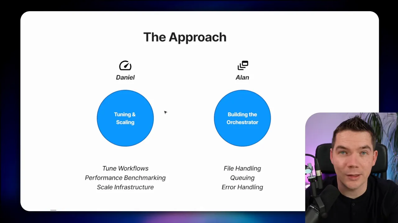
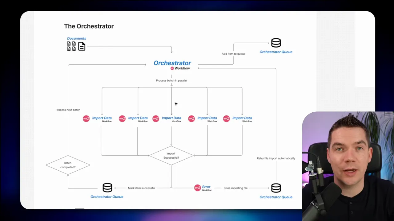
I split the work into two parts. I focused on tuning the existing RAG ingestion workflow to remove bottlenecks and make it as efficient as possible. Once the workflow ran well, I increased parallelism and capacity. My colleague built an orchestrator that could dispatch many files into the workflow in parallel and add retry logic. The orchestrator is an important piece because the main RAG workflow was originally built to process files one at a time.

My iterative approach to tuning

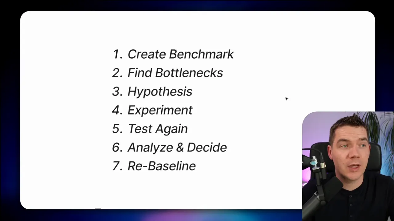
I followed a simple iterative process:

• Create a baseline benchmark and measure performance.
• Inspect execution logs to find the slow nodes.
• Form hypotheses about causes and possible fixes.
• Implement targeted changes or alternative approaches.
• Retest and compare against the baseline.
• Keep changes that provide real improvements and roll back ones that don’t.
• Repeat until the result meets the needs and the effort no longer justifies further gains.

This structured loop kept me focused. It also made it much easier to see which experiments had an impact and which didn’t.

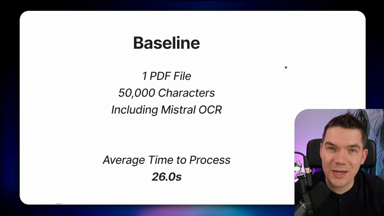
Benchmark: the baseline

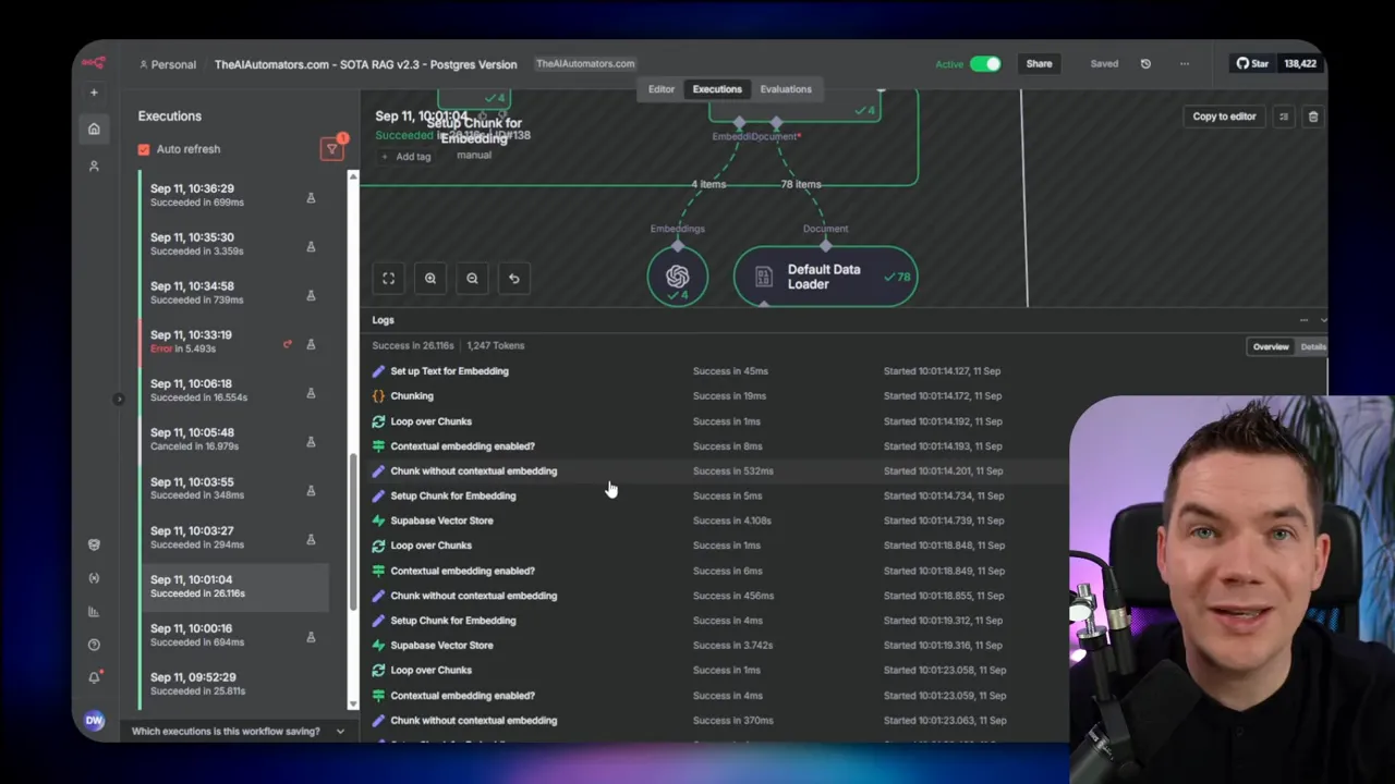
I needed a consistent test file. I used a 24-page PDF instruction booklet (about 50,000 characters) that included both readable text and images requiring OCR. I ran that file repeatedly through the importer with the workflow configured as it originally was. The average time was 26 seconds per file. At that rate you can only process roughly 120 files per hour — far from my goal.

All performance measurements I describe here relate to that baseline and to subsequent tests using multiple files. Wherever I changed the test file mix or configuration, I documented it so I could compare apples to apples.

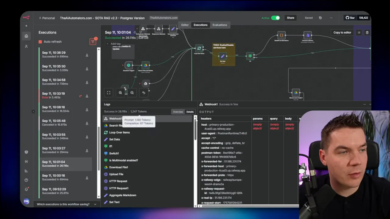
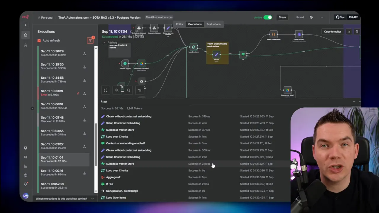
How I found bottlenecks

n8n provides an execution history with timing information per node. This is where you need to spend time. For a long workflow, the slowest nodes stand out. In one baseline run I saw:

• Download from Google Drive: ~2 s
• Upload to Mistral (OCR): ~1.5 s
• Metadata extraction with GPT-4 Mini: ~1.7 s
• Upsert into Supabase: 2–4 s across several upserts

Seeing those numbers made it clear where I should test changes first.

Tuning experiment #1: batch files in the loop

The first idea I tried was to process multiple files in the top-level loop rather than one at a time. The loop node can be configured to accept batches — for example, 5, 10, or 20 files per iteration. I hoped parallelizing within a single workflow execution would give a large speed-up.

The reality was more complex. The workflow had nested loops and lots of mappings between nodes. When you increase the batch size in an n8n “loop over items” node, you often need multiple merge nodes and complex mapping logic to keep items aligned with the outputs of subsequent nodes. For example, when fetching metadata fields from a database, the number of results may differ from the number of input files. That mismatch forces extra merging logic.

I tested several batch sizes:

• Batch size 1 (sequential) — baseline.
• Batch size 5 — roughly a 10% improvement.
• Batch size 10 — no meaningful improvement.
• Batch size 20 — server crashed due to memory usage while downloading many binary files at once.

The crash was predictable. Downloading 20 PDF binaries in parallel used too much RAM. You can offload binary data to disk rather than keeping it in memory, but refactoring for that was time-consuming and added complexity. That led me to deprioritize this approach for now.

Later I learned a hard lesson: when I removed another bottleneck, this batch-work approach became much more effective. So if you get a small improvement early, re-baseline after other major wins. Early tests that look marginal can become significant after you fix larger issues.

Tuning experiment #2: increase chunk batch size

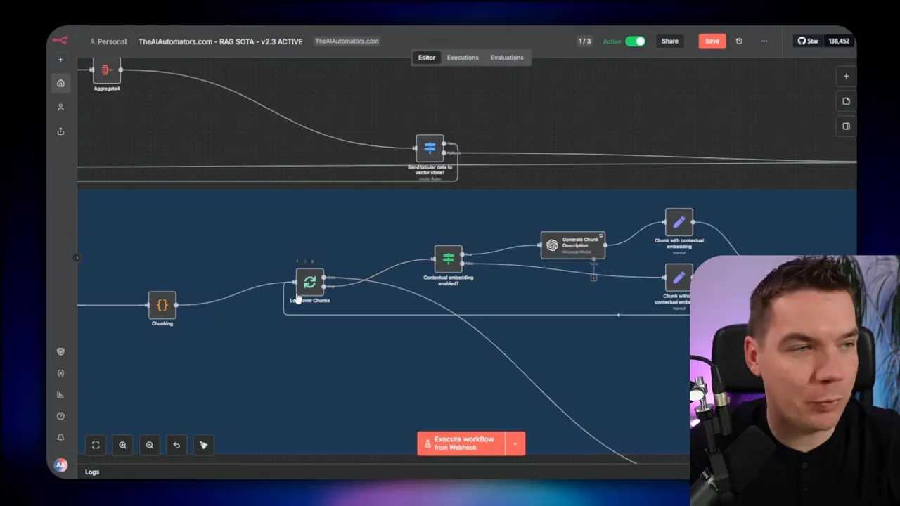
The next hotspot was the nested chunk processing loop. I use a custom chunking function that splits a document into chunks and then, for each chunk, calls an LLM to generate a short contextual snippet that sits at the start of each chunk. This snippet helps ground the chunk in the document and improves retrieval quality, but calling an LLM for every chunk doesn’t scale well.

The chunk loop originally processed small batches, largely to keep LLM rate-limit and latency manageable. I hypothesized that increasing the chunk batch size would reduce the number of LLM calls and raise throughput. I tested raising chunk batch size from 20 to 200.

The result: around a 20% improvement in processing time per file. That was a clear win. But it came with a trade-off. The contextual snippet for each chunk came from an LLM, and batching too aggressively can reduce the prompt design flexibility and increase error surface area. For now, I kept the larger batch size and noted that this pattern (one LLM call per chunk) may not be ideal for truly massive scaling. For high-scale systems, I decided to avoid per-chunk LLM calls where possible.

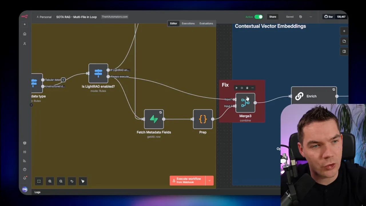
Tuning experiment #3: optimize vector store inserts

The single biggest win came from rethinking how I wrote chunks to Supabase. The default vector store node in n8n supports chunking and a data loader. I was manually generating chunks and inserting them into the Supabase documents table using the vector store node. The upsert times in the logs showed several 3–4 second delays at this stage. That hinted the vector store step was a bottleneck.

I tested three approaches:

1. Let the native vector store node accept the full document and do the splitting internally.
2. Keep custom chunking and pass chunks into the vector store node (like I was doing).
3. Keep custom chunking but bypass the vector store node and insert directly into the Supabase documents table via SQL.

Option 1 and option 2 performed similarly. Option 1 (native splitting) was reasonably fast, but it lacked support for the contextual embedding pattern I needed. Option 2 was slow with my custom chunking. I observed that the standard module repeatedly fetched or computed metadata per chunk even when the metadata was static per document. That repeated work multiplied latency.

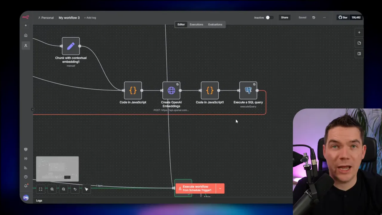
I moved to option 3. I replaced the vector store node with a direct SQL insert into the Supabase Postgres documents table. I used a transaction-oriented approach and batch inserts where appropriate. ChatGPT helped me craft the SQL to match the documents table schema. The results were immediate: the insert step dropped from multiple seconds to around half a second. Generating embeddings still took about 1.2 seconds, but overall the vector store stage became much faster. That single change gave me roughly a 55% speed improvement on the per-file processing time.

Important note: directly inserting into the Postgres documents table bypasses the convenience of the native node. It also comes with operational trade-offs. You need to ensure the rows are inserted in the correct format and that you keep the structure consistent with how your vector store expects to retrieve and search. You might also hit database connection limits at scale. For my tests, I used a dedicated connection pooler for Postgres to handle many concurrent connections. This required extra setup and monitoring.

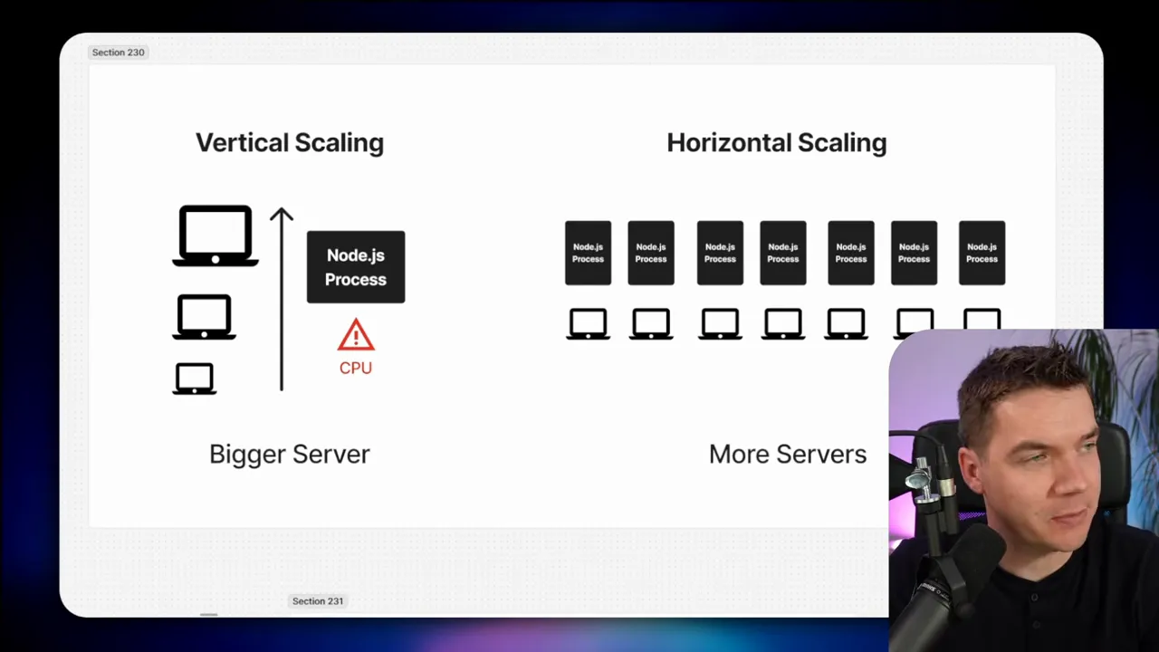
Scaling: vertical vs. horizontal

Once the workflow ran faster per file, I scaled the infrastructure. There are two common scaling strategies:

• Vertical scaling: add CPU, RAM, and disk to a single server.
• Horizontal scaling: add more servers and distribute the load across them.

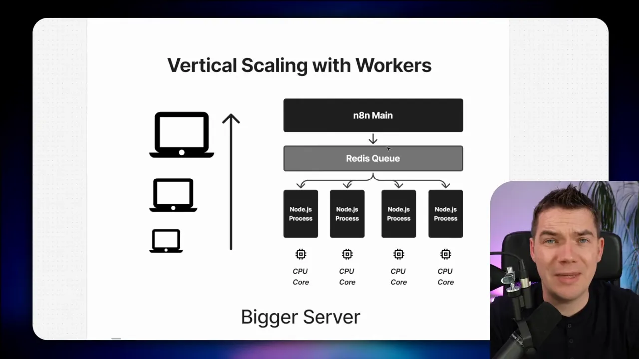
n8n runs on Node.js. Node apps are single-threaded. That means one n8n process can use only one CPU core for synchronous JS execution. You can run multiple n8n worker processes on the same machine to effectively use more CPU cores. That approach is often called running in queue (or worker) mode. Each worker polls a Redis queue for jobs and processes execution items.

For larger scale, horizontal scaling works well. You run an “n8n main” instance that handles the editor, web UI, and API. The main instance enqueues jobs into Redis. Multiple worker instances, possibly across multiple servers, then poll Redis and process jobs. Each worker is a headless n8n instance sharing the same database and encryption key as the main instance so it can complete executions correctly.

Workers, Redis, concurrency

When running in queue mode, a few parameters matter:

• Number of workers: how many n8n worker processes you run across your fleet.
• Concurrency per worker: how many executions each worker can handle at the same time. The default is often 10.
• Queue design: how jobs get enqueued and how the orchestrator triggers executions.

If you run four workers and each worker has concurrency set to 10, that cluster can process up to 40 jobs concurrently. That parallel capacity is what unlocks high throughput. But it also changes how you design upstream systems. Some third-party APIs will rate-limit you, and some database setups need connection poolers to handle many concurrent DB clients.

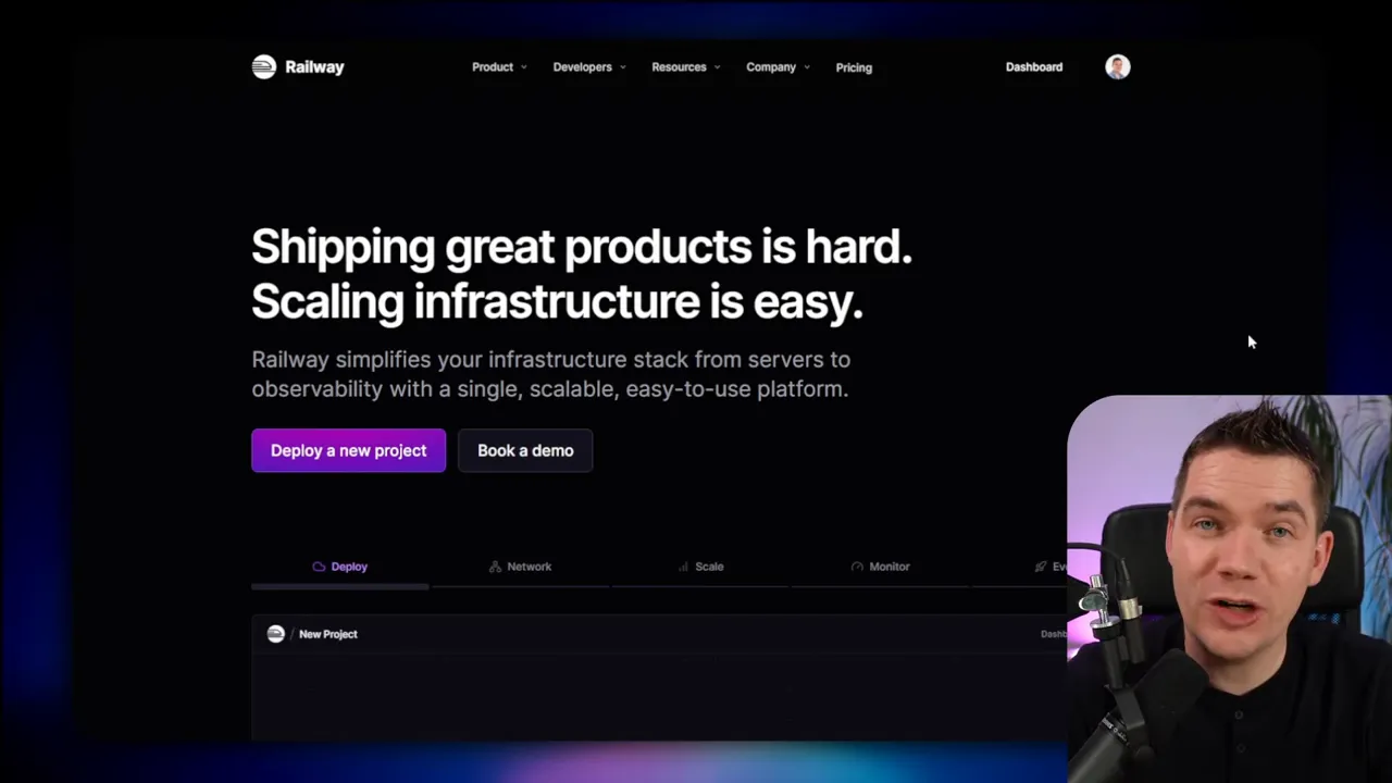
Using Railway as a simple testbed

For testing I used Railway. It’s not the only option, but it provides a quick template that deploys an n8n main instance, a worker, Postgres, and Redis. You can replicate workers in the Railway UI to add more capacity rapidly. Railway also supports replicas, which appear to run multiple instances behind a load balancer. That made it easy to ramp capacity without touching Docker or Kubernetes configs.

How the orchestrator works

The main RAG workflow alone enqueues a single execution. If you trigger the entire 90-node workflow once, that’s one job for the workers. To make real parallelism, I needed a system that pushed many individual files into the Redis queue as separate executions.

My colleague built an orchestrator workflow. The orchestrator fetches files from a file host and triggers the RAG ingestion workflow repeatedly by calling its webhook. There are two important implementation details that made this fast and resilient:

• Triggering the RAG workflow via webhook is faster than using a sub-execution. The webhook returns an execution ID immediately, so the orchestrator can continue looping without waiting for the file to be processed.
• The orchestrator adds an additional tracking queue that records success or failure for each execution. If a job fails, the system automatically retries it a limited number of times (we used up to three retries). This resilience is crucial when third-party APIs occasionally fail or rate-limit under load.

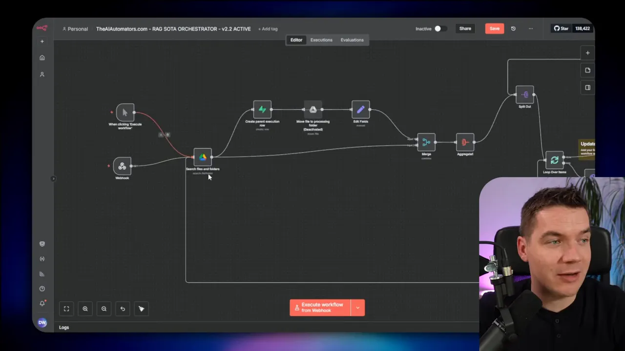
The orchestrator pattern decouples the act of scheduling imports from the work of executing them. The orchestrator can queue thousands of small jobs quickly. Then the worker fleet processes them in parallel. This design also allows the orchestrator to implement retry and backoff policies without complicating the main RAG workflow.

Real-world scaling tests and surprising results

With the orchestrator in place, I began scaling tests and tuning parameters. I ran many experiments. I’ll highlight the most important ones and what I learned from each.

Test 1: two workers, batch size 12, Mistral OCR enabled

I started with two workers and a file batch size of 12. For the test I fed 20 PDF files through the orchestrator. The average processing time per file dropped from 9.2 seconds to 4.1 seconds — roughly a 55% improvement. That looked promising.

However, the numbers didn’t fully add up. Each worker has concurrency set to 10. Two workers therefore could process up to 20 files at once. In that scenario, processing 20 files should have taken roughly the same time as processing one file. The expected total duration should have been close to the single-file latency. In practice, the improvement didn’t match the theoretical capacity.

The reason was subtle: concurrency doesn’t always equate to parallelism when other parts of the pipeline are sequential or when the orchestrator introduces sequential steps. I needed to check the entire flow end to end, not just the workers.

Test 2: remove Mistral to find the bottleneck

I suspected Mistral OCR because each file required an OCR call. I removed Mistral from the pipeline to see whether that would move the needle. The time improved only slightly, from 4.1 seconds to 3.8 seconds. Mistral wasn’t the principal bottleneck at this stage.

That led me back to the orchestrator. My colleague had written the orchestrator to move each file into a processing folder before triggering the import execution. That move was sequential and slow. The orchestrator was spending significant time moving files rather than simply queuing executions.

To fix that, I disabled the file-moving step in the orchestrator and moved that responsibility into the RAG ingestion flow itself. This change allowed the orchestrator to fire off webhooks quickly and let workers handle file movement and processing in parallel.

Test 3: re-test with orchestrator change

Removing the sequential file move dropped processing time dramatically. For the 20-file run, average time per file went down to about 1.1 seconds. That was a major improvement and an excellent illustration that the orchestrator design matters as much as worker count.

At that point I increased the batch size the orchestrator sent into the queue. I had four workers with replicas available. With concurrency set to 10, I had theoretical capacity to process 80 files at once. I raised the file batch size to 50 and tested again. The file processing time dropped to about 0.7 seconds per file. That meant the system was over-provisioned for the test dataset and could safely run on fewer resources if cost was a concern.

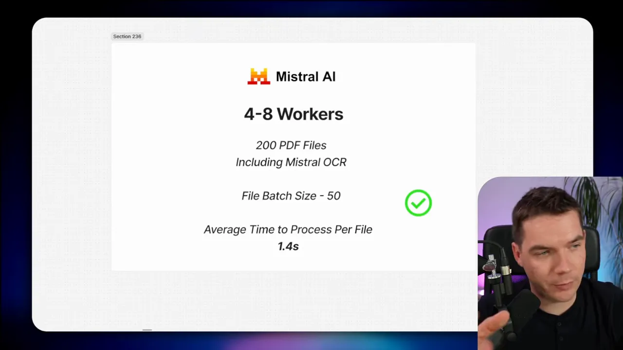
Test 4: re-enable Mistral and scale up

Next I re-enabled Mistral OCR because OCR is important for high-quality embeddings. I tested with 200 files and a file batch size of 50. The average time per file increased from 0.7 s to 1.4 s. That is still very fast given the document complexity. Many of those PDFs were up to 50 pages long, and Mistral handled concurrent OCR extremely well. Across multiple runs, results were consistent: whether I sent 20 files or 200 files, the average hovered around 1.4 seconds per file with Mistral enabled and the cluster configured for high parallelism.

Final performance numbers and what they mean

After tuning and scaling, these were the headline numbers I achieved in testing:

• Overall processing time per file: roughly 0.7 seconds (without OCR) and 1.4 seconds (with Mistral OCR) depending on test conditions.
• Throughput: about 5,000 PDF files per hour in the test environment when fully scaled up.
• Data scale in the largest test: ~10 GB of PDF data resulting in ~250,000 chunks in the vector store.
• Total tuning time: about 100 hours of iterative testing and infrastructure adjustments.

These numbers are a combination of workflow-level optimizations and infrastructure scale. Changing a single bottleneck without scaling the rest of the system would not produce the same gains. Likewise, scaling servers without removing bottlenecks yields limited improvements and can even slow things down.

Key lessons I learned

I learned many lessons during this project. Here are the most important ones, with practical advice you can apply immediately.

1. Use a systematic approach

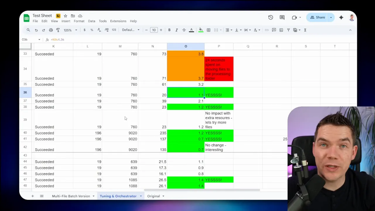
Random tweaks rarely work. I used a structured Google Sheet to record configuration settings, test runs, and metrics. Every time I changed a parameter, I documented the results. That made it simple to compare the impact of each experiment. I recommend this seven-step process:

1. Benchmark your current flow using a representative test file.
2. Inspect execution logs and identify the highest-latency nodes.
3. Generate hypotheses about likely causes and possible fixes.
4. Implement one change at a time to isolate effects.
5. Retest and compare against the baseline.
6. Decide whether to keep or revert the change.
7. Repeat until improvements plateau or the effort no longer justifies further gains.

2. Fix bottlenecks before throwing resources at the problem

I added workers and CPU, but scaling hardware did not always help until I removed the real bottlenecks. For example, switching to many workers while the orchestrator still moved files sequentially didn’t yield the expected gains. Once I removed the sequential steps, extra workers produced the speed increases I expected.

3. Third-party systems can be the real limit

n8n workflows often depend on external APIs. Those APIs can throttle or rate-limit you. If you push too much at once, the third-party service will slow you down. A useful approach is to avoid APIs where feasible. For Supabase, I wrote directly to the Postgres documents table to avoid repeated metadata lookups and to get faster inserts. For file storage, I moved from using the Google Drive node to an SFTP server to avoid flaky cached responses and node-specific issues. These changes require more operations work and monitoring, but they can pay off at scale.

4. Watch out for memory and binary handling

Downloading many binaries in parallel can eat RAM quickly. When I tried to process 20 files in parallel within one execution, the server ran out of memory. You can avoid this by offloading binary data to disk instead of keeping it in memory, or by reducing parallel binary downloads per process and relying on multiple worker processes to spread the load.

5. Native nodes are convenient, but not always optimal

n8n’s native vector store node is easy to use. But in my case, the native node repeatedly fetched metadata for each chunk when the metadata was static per document. That repeated work hurt performance. Replacing that step with a direct SQL insert gave a much faster path and allowed me to keep my contextual snippet pattern. Before making a direct DB change in production, audit the expected schema, test on a staging DB, and monitor connection counts.

6. Don’t ignore the orchestrator

The orchestrator is the gatekeeper of parallelism. If the orchestrator introduces sequential tasks or chokepoints, workers will be starved and parallel improvements will stall. Keep the orchestrator lightweight and focused on dispatching tasks quickly. Delegate heavy work to the workers.

7. Expect diminishing returns

At some point, the cost of cutting a few hundred milliseconds from per-file latency isn’t worth the effort. I reached a point where per-file time was about 0.7 seconds without OCR and 1.4 seconds with OCR. I could have continued trimming fractions of a second, but the law of diminishing returns suggests it’s often better to stop when the system is stable and cost-effective.

8. Self-hosting may become necessary

If you scale past a certain point, hosted services can become expensive or limiting. For extreme scale, you may need to self-host components: n8n, the database, the file server, and possibly the vector store. Self-hosting gives you full control over connection poolers, resource allocation, and retention policies, but it adds operational overhead.

Practical checklist and recommendations

If you want to follow the same path, here’s a compact checklist you can use when tuning and scaling your own RAG ingestion workflows:

• Pick a representative benchmark file and test set.
• Record every change and result in a spreadsheet.
• Inspect n8n execution logs per node for timing breakdowns.
• Identify expensive repeated operations (e.g., per-chunk metadata fetches).
• Consider replacing slow native nodes with direct DB calls if necessary and safe.
• Avoid storing binary files in memory when processing many in parallel.
• Design an orchestrator that enqueues jobs quickly and delegates heavy work to workers.
• Use Redis queue and multiple worker instances; tune concurrency per worker.
• Monitor third-party API limits and add backoff/retry logic or move to a self-hosted alternative.
• Test at progressively larger batch sizes and re-baseline after each major fix.
• Stop when the system is stable and meets your performance/cost objectives.

Some operational details worth noting

Below are practical details that saved me time during the project. I summarize them as short tips you can apply immediately.

Use webhooks for fast enqueueing

Triggering the RAG workflow via its webhook is faster than invoking a sub-execution. The webhook offers an immediate execution ID you can track. The orchestrator can then continue dispatching files without waiting for the full execution to complete.

Keep metadata static where possible

If metadata is identical across chunks in a document, don’t recompute or refetch it per chunk. Embed the static metadata in the SQL insert or pass it once at the document level so vector store writes don’t perform unnecessary lookups.

Batch DB writes

When writing many small rows, consider batching inserts or using a transaction to reduce overhead. Also be mindful of the database’s max connections; use a pooler if you expect many concurrent clients.

Be careful with LLM calls per chunk

Calling an LLM for each chunk can improve retrieval quality but won’t scale easily. Consider alternatives like document-level snippets, algorithmic context extraction, or using a smaller, cheaper LLM in batched mode.

Monitor connection and memory usage

When running many workers, monitor database connections and memory use on each worker host. Connection limits and memory exhaustion are common failure modes at scale.

Final notes about trade-offs

Every design choice came with trade-offs. I kept the contextual embeddings because they improved retrieval, but I had to change how inserts were performed to keep performance acceptable. I wanted the convenience of native nodes, but I accepted extra operational complexity (direct SQL and a connection pooler). I pushed parallelism with many workers, but only after eliminating serial bottlenecks in the orchestrator and the main workflow.

Ultimately, the combination of careful profiling, targeted code and node changes, and a proper worker-orchestrator architecture produced a system that scales to thousands of documents per hour while preserving high-quality OCR and embeddings.